Statistical Inference Fundamentals: From Data to Decision
A typical statistical analysis follows these steps:
- Define the problem: What specific truth do we want to uncover? (For example: "What is the true efficacy rate of the new drug?")
- Plan data collection: How will we gather relevant data? (For example: design a clinical trial or survey.)
- Analyze the data: Use statistical models to analyze data and draw inferences.
- Quantify uncertainty: How reliable is our inference?
The concept of a "model" is essential here. A model is a set of assumptions about the random process that generates our data. If our model's assumptions are flawed, our conclusions become unreliable. As one professor aptly put it: "If I collect shoe sizes of all students in my class to predict their GPA, it's basically impossible." This highlights a fundamental rule: data must be relevant to the question. No amount of sophisticated analysis can extract meaningful answers from irrelevant data.
The reliability of statistical conclusions also depends heavily on sample size. Consider a claim that new $250 running shoes significantly improve performance. If a New York Times dataset contains 500,000 running times across 50 different shoe models and consistently ranks this model first, the evidence is compelling. Large data volume speaks for itself. In contrast, if only a handful of runners wearing this shoe run faster, it's easily coincidence. Large samples provide credibility for our findings; small samples require more cautious interpretation.
Modeling Binary Outcomes with Bernoulli Distribution
The simplest yet foundational statistical model is the Bernoulli model, which describes random phenomena with only two possible outcomes. A Bernoulli random variable takes value 1 ("success") or 0 ("failure"). Examples are everywhere: flipping a coin (heads/tails), exam results (pass/fail), or patient recovery (cured/not cured).
The Bernoulli distribution is defined by a single parameter p, the probability of "success." We write:
$P(\text{outcome} = 1) = p$ and $P(\text{outcome} = 0) = 1-p$.
When we say a random variable $X$ follows a Bernoulli distribution with parameter $p$, we write $X \sim \text{Bernoulli}(p)$.
The Bernoulli model is the cornerstone of statistics. Many complex models build upon it. For example, if we want to know the true cure rate (parameter p) of a new drug, we can model each patient's outcome ($R_i$) as a Bernoulli variable: $R_i=1$ if cured, 0 otherwise. The total number of cured patients in a trial of 100 is the sum of these Bernoulli variables, following a binomial distribution $\text{Binomial}(n=100, p)$.
Encoding outcomes as 0/1 also simplifies computation. A key property of a Bernoulli variable is that its expected value (or mean) equals its success probability: $E[R_i] = 1 \cdot p + 0 \cdot (1-p) = p$.
This means if we have $n$ independent observations, the sample mean $\hat{p} = \frac{1}{n}\sum_{i=1}^n R_i$ is simply the proportion of successes in our sample. This sample proportion is our natural estimate of the true probability $p$.
Example: The Kissing Study
An amusing study observed whether kissing couples tend to tilt their heads to the right or left. Researchers collected data on $n=124$ couples, recording rightward tilt as "1" and leftward as "0". In this dataset, 80 couples tilted right.
Our estimate of the proportion tilting right is: $\hat{p} = 80/124 \approx 0.645$
This suggests about 64.5% of couples tilt right. This number exceeds 50%, but is it significantly greater than 50%? Is this a true preference or just random coincidence in our sample? The Bernoulli model provides a framework for answering this question, which we'll explore shortly.
The i.i.d. Assumption: The Foundation of Statistics
When building models, one of the first questions to ask is whether data can be treated as i.i.d. (independent and identically distributed). This assumption is the foundation of many classical statistical theorems.
Independence
Independence means each observation is unrelated to all others; the outcome of one trial does not affect another.
- Good example: Successive rolls of a fair die, or responses from a random-digit-dial telephone survey.
- Bad example: Daily stock prices (today's price correlates with yesterday's), "likes" on social media (friends' behavior influences one another), or blood pressure readings from family members (shared genetics and lifestyle).
When independence is violated, standard tools like the Law of Large Numbers and Central Limit Theorem cannot be directly applied. More advanced models (such as time series, network models, or mixed-effects models) are needed.
Identical Distribution
This means all observations come from the same underlying probability distribution with the same parameters.
- Good example: Repeatedly flipping the same coin, always with probability 0.5 of heads. Random sampling from a large national population for a political poll.
- Bad example: In the kissing study, if data were collected at different times in an airport, demographics (and thus behavior) might change, violating the assumption. Similarly, if a study about handedness preference mixed left-handers and right-handers without accounting for it, the data would not come from a single, uniform distribution.
In practice, if we identify distinct subgroups with different characteristics, we should use more sophisticated techniques, such as stratified modeling, rather than assuming a single, uniform distribution.
The i.i.d. assumption is a powerful simplification. Good experimental design—using randomization, blinding, and careful sampling—often aims to create conditions where data can reasonably be treated as i.i.d.
Properties of the Sample Mean
The sample mean (or sample average) is the most fundamental statistic. For i.i.d. data, it serves as a natural estimator of the population mean. For our Bernoulli sample, the sample mean is $\hat{p}$.
Expectation (Unbiasedness)
The expected value of the sample mean $\hat{p}$ is the true population proportion $p$. $$E[\hat{p}] ;=; E!\Big[\frac{1}{n}\sum_{i=1}^n R_i\Big] ;=; \frac{1}{n}\sum_{i=1}^n E[R_i] ;=; \frac{1}{n}\cdot n p ;=; p.$$ This property makes $\hat{p}$ an unbiased estimator of $p$. On average, our estimate hits the true value.
Variance (Precision)
Of course, no single experiment will perfectly match the expectation. The variance of the sample mean tells us how much it is expected to fluctuate around the true value. For independent $R_i$ with variance $\text{Var}(R_i) = p(1-p)$, the variance of $\hat{p}$ is: $$\operatorname{Var}(\hat{p}) ;=; \operatorname{Var}!\Big(\frac{1}{n}\sum_{i=1}^n R_i\Big) ;=; \frac{1}{n^2}\sum_{i=1}^n \operatorname{Var}(R_i) ;=; \frac{1}{n^2}\cdot n,p(1-p) ;=; \frac{p(1-p)}{n}.$$ This formula is extremely important. It shows that the variance of our estimate decreases as sample size $n$ increases. This is the mathematical foundation of the power of large samples: they yield more stable and precise estimates.
Law of Large Numbers and Central Limit Theorem
These properties lead to two of the most important theorems in statistics:
Law of Large Numbers (LLN): As sample size $n$ grows arbitrarily large, the sample mean $\hat{p}$ converges to the true population mean $p$. This guarantees that with sufficient data, our estimate will be arbitrarily close to the truth.
Central Limit Theorem (CLT): For sufficiently large sample size $n$, the distribution of the sample mean $\hat{p}$ is approximately normal, regardless of the distribution of the original data: $$\hat{p} \approx N!\Big(p,;\frac{p(1-p)}{n}\Big)$$ The CLT is powerful because the normal distribution is well understood, allowing us to compute probabilities and construct confidence intervals for our estimates.
Example: Cryo-EM (Cryogenic Electron Microscopy)
The power of averaging i.i.d. data is perfectly exemplified in cryo-EM, a revolutionary technique for determining the 3D structure of biological molecules. Scientists freeze and image hundreds of thousands of individual protein particles, but each image is extremely noisy.
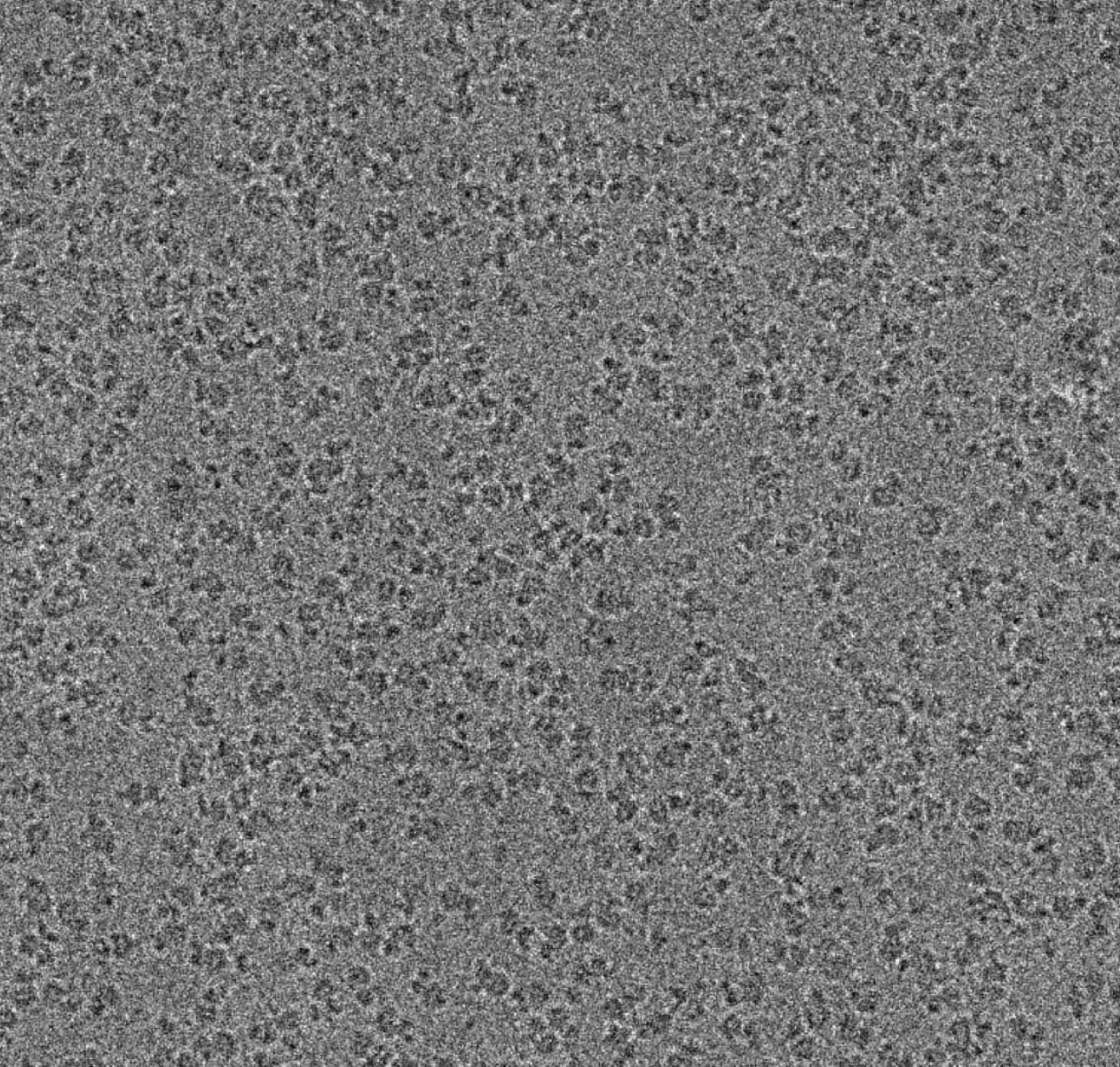
To reconstruct the structure, images are aligned and then averaged. Because the noise in each image is random and independent, it cancels out during averaging. However, the weak underlying signal of the protein is consistent and is enhanced during averaging.
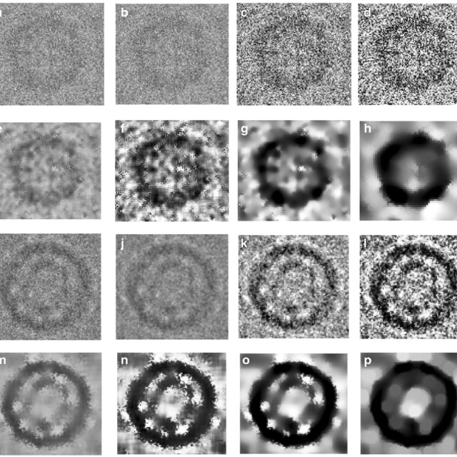
This is a direct application of the principles we've discussed:
- Independence: The noise in each image is random, uncorrelated with other images.
- Identical distribution: All particles are the same protein, so the underlying signal is identical.
- Law of Large Numbers: By averaging tens of thousands of images, random noise averages to zero.
- Variance reduction: Noise variance in the final image is reduced by a factor of $n$, dramatically improving the signal-to-noise ratio.
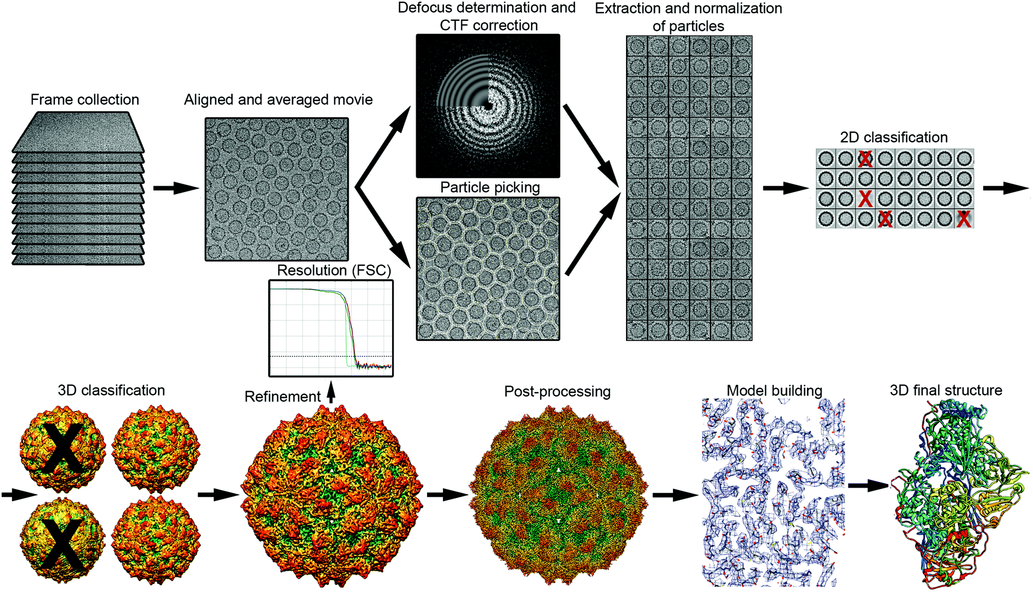
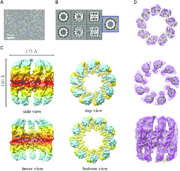
The result is a high-resolution 3D map of the molecule, an achievement made possible by the fundamental principle of statistical averaging.
Theory and Simulation: Two Ways to Quantify Error
How do we quantify uncertainty in our estimate $\hat{p}$? We have two main tools: theoretical formulas and computational simulation.
1. Analytical Method (Theory)
Using probability theory, we can derive exact formulas for error measures. As we saw, the standard deviation of $\hat{p}$, called the standard error, is $\sigma_{\hat{p}} = \sqrt{p(1-p)/n}$. This gives us a direct measure of the size of estimation error.
We can use this, usually combined with the Central Limit Theorem, to answer probability questions. For example: "What is the probability our estimate $\hat{p}$ differs from the true value $p$ by more than 10%?" This can be expressed as $P(|\hat{p} - p| > 0.1)$. For large $n$, we can use the normal distribution to approximate this.
This analytical method is powerful because it gives us exact, quantitative answers about uncertainty.
2. Numerical Method (Simulation)
When theoretical formulas become too complex or unwieldy, we can use Monte Carlo simulation. The idea is to use a computer to simulate our experiment many thousands of times under specific assumptions (such as assuming the true $p=0.5$).
For the kissing study, we could simulate 100,000 experiments, each with 124 "couples". In each simulation, we generate 124 random 0/1 values (with $p=0.5$) and compute a simulated $\hat{p}$. By plotting a histogram of these 100,000 simulated $\hat{p}$ values, we obtain an empirical distribution showing what range of results we might expect if the true proportion were 50%.
If our observed value ($\hat{p} = 0.645$) falls in a very low-density region of this histogram (that is, in the tail), it suggests our initial assumption (that $p=0.5$) is probably wrong.
Simulation is intuitive and flexible, but it depends on correctly modeling the data-generating process and requires substantial computation to accurately estimate very small probabilities.
Hypothesis Testing and Statistical Significance
Let's return to the kissing study. Our observed proportion is $\hat{p} = 0.645$. Is this strong evidence to conclude that people have a preference for tilting right? This is the question of hypothesis testing.
The framework works as follows:
State the hypotheses:
- Null hypothesis ($H_0$): This is the scenario of "no effect" or "no difference". Here, $H_0: p = 0.5$ (no preference for tilting right or left).
- Alternative hypothesis ($H_1$): This is what we wish to establish. Here, $H_1: p > 0.5$ (preference for tilting right).
Calculate the test statistic and p-value: Our test statistic is the count of "successes" (tilting right), namely $X=80$. The p-value quantifies how extreme this result is. It is defined as the probability of observing a result at least as extreme as our data, assuming the null hypothesis is true.
In this case: $p\text{-value} = P(X \ge 80 \mid p=0.5)$.
If this p-value is very small, it means the data we observed is highly unlikely under the "no preference" assumption. This would lead us to reject the null hypothesis in favor of the alternative.
To build intuition, we can run a simulation. We assume the null hypothesis is true ($p=0.5$) and simulate the experiment many times.
import numpy as np
import matplotlib.pyplot as plt

# ---------------- user-adjustable parameters ----------------
p_true   = 0.5       # probability under H0 (no preference)
n_sample = 124       # couples per experiment
N_sim    = 100_000   # how many experiments to simulate
obs_hatp = 0.645     # the real sample proportion we observed
# ------------------------------------------------------------

rng   = np.random.default_rng(seed=2025)
data  = rng.binomial(1, p_true, size=(N_sim, n_sample))
hat_p = data.mean(axis=1)

# empirical p-value: proportion of experiments where hat_p ≥ observed value
p_empirical = np.mean(hat_p >= obs_hatp)

# ---------- plot ----------
plt.figure(figsize=(6,4))
plt.hist(hat_p, bins=40, density=True, edgecolor="black", alpha=0.9, color="#F5A623")
plt.axvline(obs_hatp, ls="--", lw=2, color="#FF6F00", label=fr"$\hat p_{{obs}}={obs_hatp}$")
plt.title(fr"Monte-Carlo distribution of $\hat p$ ($n={n_sample},\,p={p_true}$)")
plt.xlabel(r"sample proportion $\hat p$")
plt.ylabel("density")
plt.legend()
plt.tight_layout()
plt.show()

print(f"Empirical P(hat_p ≥ {obs_hatp}) = {p_empirical:.5f}")
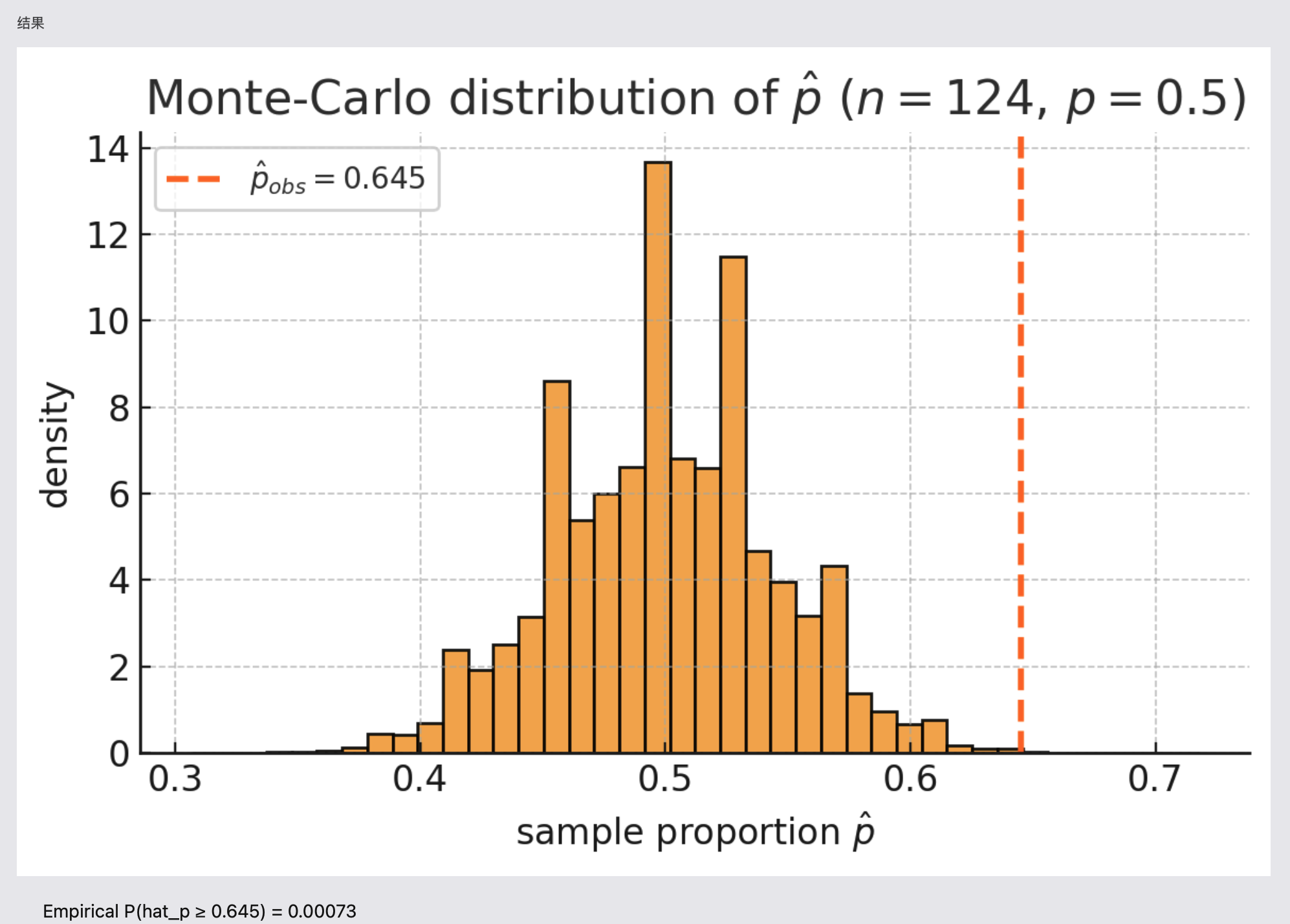
The histogram shows the distribution of sample proportions from 100,000 simulated experiments where the true preference is 50/50. Our observed value of 0.645 lies far in the right tail.
Simulated Right-Tail Probability
$\widehat{P}(\hat{p}\ge 0.645);=;0.00084;;(\text{approximately }0.084%)$
This simulated p-value is extremely small. It tells us that if there truly were no preference, the probability of seeing a result this strongly favoring the right is less than one in a thousand. Therefore, we have strong statistical evidence to reject the null hypothesis and conclude that there is indeed a true preference for tilting right when kissing.
An alternative to hypothesis testing is to construct a confidence interval. A 95% confidence interval for $p$ might be, for example, [0.56, 0.72]. This gives us a plausible range for the true value of $p$. Since this interval does not contain 0.5, it leads to the same conclusion as our hypothesis test: the true proportion is likely greater than 50%.
Principles for Collecting Good Data
The quality of any statistical conclusion is fundamentally limited by the quality of the data. The principle of "garbage in, garbage out" is critical. Here are key considerations for collecting reliable data.
Randomized experiments vs. observational studies: Prefer randomized experiments whenever possible. By randomly assigning subjects to a treatment group (e.g., receiving a new drug) and a control group (e.g., receiving a placebo), we can isolate the treatment effect and minimize confounding bias. Randomization is a powerful tool for ensuring the i.i.d. assumption holds.
Representative sampling: For observational studies, the goal is to obtain a sample that is a miniature replica of the population. Simple random sampling is ideal, though strategies like stratified sampling can be more efficient. The key is to avoid selection bias. A survey conducted only through online forums may overrepresent certain populations and not generalize to the entire population.
Sample size planning: Before beginning a study, it is wise to conduct a power analysis to estimate the required sample size. This ensures the study is large enough to detect a meaningful effect without wasting resources collecting excess data.
Avoid dependence: The data collection process itself should not introduce dependence. Survey respondents should not discuss their answers; experimental subjects should be isolated from one another. If dependence is unavoidable (such as in time series data), appropriate models must account for it.
Ethical and practical constraints: Real-world data collection is often constrained by ethics and logistics. Giving a placebo to a critically ill patient may be unethical; a perfect random sample may be too expensive. In such cases, we must find the best design within the constraints and be transparent about data limitations when reporting results.
Conclusion
Statistics is not merely a collection of formulas; it is a principled way of thinking about uncertainty and learning from the world. From framing the problem and designing experiments to building models and quantifying uncertainty, each step is essential. By understanding core assumptions like i.i.d. and fundamental properties of estimators, we build confidence in our conclusions.
The journey from simple Bernoulli trials to complex real-world problems like cryo-EM reconstruction rests on these foundational ideas. As we explore more advanced models, we must always return to first principles: understand your data source, make explicit your assumptions, and be honest about the limits of your conclusions. Carefully designed data collection, paired with sound analysis, is key to transforming information into insight.