A Deeper Dive into Probability: From Convergence to Core Concepts

Almost Sure Convergence: The Strongest Form

Almost sure convergence means that with probability 1, the random variable sequence $X_n$ converges to $X$ on all sample paths in the probability space. When $n$ is sufficiently large, $X_n$ gets arbitrarily close to $X$ and stays close forever.

For coin flipping, this is the Strong Law of Large Numbers: the sample proportion of heads almost surely converges to the true probability 0.5. This is the strongest form of convergence and implies all other types.

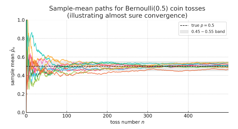
The figure above (10 colored curves) illustrates almost sure convergence:

Each curve represents one complete experiment—repeatedly flipping a fair coin, where the x-axis shows the number of tosses $n$ and the y-axis shows the proportion of heads $\hat{p}_n$ in the first $n$ tosses.

• Black dashed line: True probability $p=0.5$
• Gray band: The 0.45–0.55 interval, representing typical "settling" behavior

Key observations:

1. Initially, fluctuations are enormous (some curves even reach 0 or 1)
2. As $n$ increases, all paths stabilize and remain within the gray band
3. They never stray far from 0.5 again—this is the Strong Law of Large Numbers:

$$\mathbb{P}\left(\lim_{n\to\infty}\hat{p}_n = 0.5\right) = 1$$

If we could draw infinitely many paths, almost every one would converge this way. Only paths with probability 0 might oscillate forever—but you'd essentially never observe them.

Convergence in Probability: The Practical Standard

Convergence in probability means that as $n \to \infty$, the probability that $X_n$ differs from $X$ by more than any small threshold $\varepsilon$ approaches zero: $\Pr(|X_n - X| > \varepsilon) \to 0$.

This is weaker than almost sure convergence. While $X_n$ is usually very close to $X$ for large $n$, occasional deviations are still possible. The Weak Law of Large Numbers proves that sample means converge in probability to their expected values.

A Classic Counterexample: Consider $X_n$ that takes value 1 with probability $1/n$ and 0 otherwise. Then $\Pr(X_n = 1) = 1/n \to 0$, so $X_n \xrightarrow{p} 0$ (convergence in probability). However, since $\sum_n 1/n$ diverges, there will almost surely be infinitely many moments where $X_n = 1$, meaning the sample paths don't actually converge to 0. This shows that convergence in probability doesn't guarantee almost sure convergence.

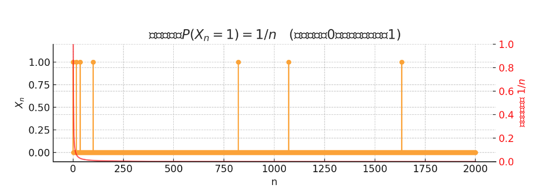
The figure shows yellow spikes representing the random variable $X_n$—mostly taking value 0, but occasionally (with probability $1/n$) jumping to 1. The red curve shows how this probability $1/n$ decreases with $n$.

• As $n$ increases, the probability of getting 1 becomes smaller, satisfying: $$\Pr(|X_n-0|>\tfrac{1}{2}) = \Pr(X_n=1) = \tfrac{1}{n} \longrightarrow 0$$ This confirms convergence in probability: $X_n\xrightarrow{p}0$

• However, observing individual paths reveals: The spikes become sparser but never disappear—no matter how large $n$ gets, 1 will still occasionally appear, so sample paths don't truly converge to 0.

This demonstrates that convergence in probability ≠ almost sure convergence.

Convergence in Distribution: The Weakest Form

Convergence in distribution means the cumulative distribution function of $X_n$ converges to that of $X$. The probability distributions gradually become similar in shape, but individual realizations need not be close.

This is the weakest form of convergence. The Central Limit Theorem is the prime example: regardless of the original distribution (as long as variance is finite and observations are i.i.d.), the standardized sample mean converges in distribution to a standard normal distribution.

Key Relationship: Almost sure convergence $\implies$ convergence in probability $\implies$ convergence in distribution. The reverse implications generally don't hold, as our counterexamples demonstrate.

When Convergence of Moments Fails

Convergence in probability doesn't guarantee convergence of variance. Consider this counterexample:

Define $X_n$ as: with probability $1/n$, $X_n = \sqrt{n}$; otherwise $X_n = 0$.

• Expectation: $\mathbb{E}[X_n] = \sqrt{n} \cdot \frac{1}{n} = \frac{1}{\sqrt{n}} \to 0$
• Variance: $\mathbb{E}[X_n^2] = n \cdot \frac{1}{n} = 1$, so $\operatorname{Var}(X_n) = 1 - \frac{1}{n} \to 1$

This $X_n$ converges to 0 in probability (since $\Pr(X_n \neq 0) = 1/n \to 0$), yet its variance approaches 1, not 0. Although extreme values become increasingly rare, they also become increasingly extreme, maintaining their contribution to the variance.

This reveals that different aspects of random variables can behave very differently during convergence, requiring careful analysis of what exactly is converging.

Part 2: The Limit Theorems That Shape Our World

The Central Limit Theorem: Why Standardization Matters

Scenario: Imagine rolling many dice and recording their sum. With 1 die, outcomes are uniform (1-6). With 2 dice, the sum distribution becomes triangular (2-12, centered at 7). With 10 dice, what happens? Intuition suggests the sum will approach a "bell curve."

This intuition is formalized by the Central Limit Theorem (CLT): the sum (or average) of many independent, identically distributed random variables, when properly standardized, converges in distribution to a normal distribution—regardless of the original distribution shape.

Why Standardization? Without standardization, the sum $S_n = X_1 + \cdots + X_n$ would have mean $n\mu$ and standard deviation $\sqrt{n}\sigma$, growing without bound. To observe a non-trivial limiting distribution, we center by subtracting $n\mu$ and scale by dividing by $\sqrt{n}\sigma$:

$$Z_n = \frac{S_n - n\mu}{\sigma\sqrt{n}} = \frac{\overline{X}_n - \mu}{\sigma/\sqrt{n}}$$

The CLT states that as $n \to \infty$, $Z_n$ converges in distribution to $N(0,1)$.

Practical Implication: For large $n$, $\Pr(|\overline{X}_n - \mu| < 3\sigma/\sqrt{n}) \approx 0.997$. This quantifies the sample mean's fluctuation: it scales as $O(1/\sqrt{n})$, with the constant "3" corresponding to the 99.7% coverage of a normal distribution.

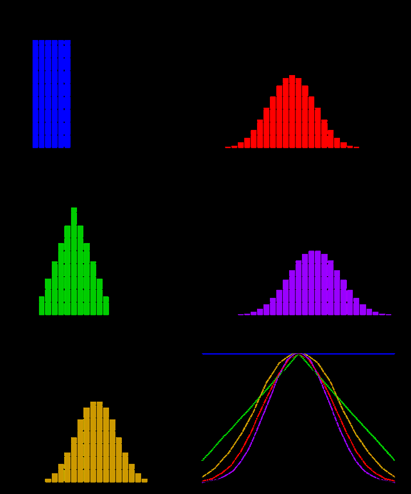
The figure shows how dice sums gradually approach a normal distribution. Top left: 1 die (uniform). Top right: 2 dice (triangular). Bottom left: 3 dice (more concentrated). Bottom right: smooth curves for 1, 2, 3, 4 dice sums with the standard normal curve overlaid (black). As the number of dice increases, the sum distribution progressively approaches normality.

Example: Suppose we measure machine part errors $X$ with unknown distribution but $\mu=0$, $\sigma=2$ mm. For $n=36$ parts, the average error $\overline{X}{36}$ satisfies $\sqrt{36}(\overline{X}{36}-0)/2 \approx N(0,1)$. Therefore, $\Pr(|\overline{X}_{36}| < 1) \approx \Pr(|Z| < 3) \approx 0.997$. The probability that the average error falls within ±1 mm is about 99.7%.

From Binomial to Poisson: The Law of Rare Events

Scenario: A website has many users $n$, each with a small probability $p = \lambda/n$ of performing some action (e.g., logging in on a given day). How many users will perform this action?

When $n$ is large and $p$ is small while $np = \lambda$ remains moderate, the binomial distribution can be approximated by a Poisson distribution. This is the law of rare events, fundamental in telecommunications, queueing theory, and reliability engineering.

Mathematical Development: Let $X_n \sim \text{Binomial}(n, \lambda/n)$. We have $\mathbb{E}[X_n] = \lambda$ and $\operatorname{Var}(X_n) \approx \lambda$ (since $(1-p) \approx 1$ when $p$ is small).

For the probability mass function: $$\Pr(X_n = k) = \binom{n}{k} p^k (1-p)^{n-k} = \frac{n!}{k!(n-k)!}\left(\frac{\lambda}{n}\right)^k \left(1-\frac{\lambda}{n}\right)^{n-k}$$

As $n \to \infty$ with fixed $k$:

1. $\frac{n!}{(n-k)!} = n(n-1)\cdots(n-k+1) \approx n^k$
2. Thus $\binom{n}{k} \left(\frac{\lambda}{n}\right)^k \approx \frac{\lambda^k}{k!}$
3. $\left(1-\frac{\lambda}{n}\right)^{n-k} \approx e^{-\lambda}$ (using the standard limit)

Combining these: $\Pr(X_n = k) \to e^{-\lambda}\frac{\lambda^k}{k!}$, which is the Poisson$(\lambda)$ probability mass function.

Rule of Thumb: If $n \geq 100$ and $np \leq 10$, the Poisson approximation to the binomial is quite accurate.

Part 3: A Practical Toolkit for Bounding Uncertainty

When we know little about a random variable's distribution, probability inequalities provide crucial bounds on tail probabilities. Different inequalities require different assumptions and provide bounds of varying tightness.

Markov's Inequality: The Most General Bound

For non-negative random variables $X \geq 0$: $$\Pr(X \geq a) \leq \frac{\mathbb{E}[X]}{a}$$

Pros: Requires only knowledge of the mean. Cons: Often provides very loose bounds.

Example: If a model's error $E \geq 0$ has $\mathbb{E}[E] = 5$, then $\Pr(E \geq 50) \leq 0.1$. This is an upper bound—the true probability might be much smaller.

Chebyshev's Inequality: Leveraging Variance Information

For any random variable with finite variance: $$\Pr(|X - \mathbb{E}[X]| \geq \varepsilon) \leq \frac{\operatorname{Var}(X)}{\varepsilon^2}$$

Advantages: Doesn't require non-negativity or boundedness, and typically gives tighter bounds than Markov when variance is known.

Example: If model error $E$ has $\mathbb{E}[E] = 0$ and $\operatorname{Var}(E) = 25$, then $\Pr(|E| \geq 10) \leq 0.25$.

Hoeffding's Inequality: The Power of Bounded Variables

For independent bounded random variables $X_1, \ldots, X_n$ with $X_i \in [0,1]$: $$\Pr(|\overline{X}_n - \mathbb{E}[\overline{X}_n]| \geq \varepsilon) \leq 2\exp(-2n\varepsilon^2)$$

This provides exponential concentration, making it extremely powerful for large $n$.

Corrected Example: To ensure the deviation probability $\varepsilon = 0.1$ is below 5%:

• Hoeffding: Solving $2e^{-2n(0.1)^2} < 0.05$ gives $n > 184$ (approximately 185 samples)
• Chebyshev: With worst-case variance 0.25, solving $\frac{0.25}{n(0.1)^2} < 0.05$ gives $n > 500$

As $n$ increases, Hoeffding's exponential advantage becomes dramatic: it provides $e^{-cn}$ decay versus Chebyshev's $1/n$ decay.

When to Use Which Inequality?

• Markov: When you only know the mean and the variable is non-negative. The bound is often conservative but better than nothing.
• Chebyshev: When you know the variance but can't guarantee boundedness. Provides universal tail control for any finite-variance distribution.
• Hoeffding: When variables are bounded and independent. Gives exponential concentration bounds, particularly powerful for large $n$. Essential in machine learning generalization analysis and A/B testing.

Part 4: Properties of Foundational Distributions

The Memoryless Property: Does Waiting Longer Improve Your Chances?

Scenario: You've been waiting at a bus stop for 30 minutes. Someone says, "Don't worry, you've waited so long that the bus must come soon!" Is this comfort mathematically justified?

If bus arrival times follow an exponential distribution, this intuition is wrong. The exponential distribution has the memoryless property: past waiting doesn't affect future waiting.

Mathematical Definition: For any $s, t \geq 0$: $$\Pr(X > s+t \mid X > s) = \Pr(X > t)$$

The probability of waiting an additional $t$ time units, given you've already waited $s$ units, equals the probability of initially waiting $t$ units.

Verification for Exponential Distribution: With $F(x) = 1 - e^{-\lambda x}$: $$\Pr(X > s+t \mid X > s) = \frac{\Pr(X > s+t)}{\Pr(X > s)} = \frac{e^{-\lambda(s+t)}}{e^{-\lambda s}} = e^{-\lambda t} = \Pr(X > t)$$

Implications:

• In queueing systems with exponential service times, the system has no "memory" of how long you've waited
• This greatly simplifies Markov process analysis
• However, most real systems exhibit aging effects, so exponential models are approximations

Working with the Standard Normal Distribution

Scenario: Statistics exams often ask: "Given $X \sim N(\mu, \sigma^2)$, find $\Pr(X \leq a)$." Since normal distributions lack closed-form CDFs, we rely on standardization and tables.

The Standardization Process:

1. Convert to standard normal: $Z = \frac{X - \mu}{\sigma}$, where $Z \sim N(0,1)$
2. Rewrite the probability: $\Pr(X \leq a) = \Pr\left(Z \leq \frac{a - \mu}{\sigma}\right)$
3. Use the standard normal table to find $\Phi(z) = \Pr(Z \leq z)$

Key Techniques:

• For negative values: Use symmetry: $\Pr(Z \leq -z) = \Pr(Z \geq z) = 1 - \Pr(Z \leq z)$
• For intervals: $\Pr(a < X < b) = \Pr(X \leq b) - \Pr(X \leq a)$
• Remember the 68-95-99.7 rule: Approximately 68%, 95%, and 99.7% of data falls within 1, 2, and 3 standard deviations, respectively

Part 5: The Linear Algebra Backbone

Many advanced probability concepts, especially in multivariate settings or machine learning applications like Principal Component Analysis, rely heavily on linear algebra. Understanding eigenvalues, eigenvectors, and how rank and determinant relate to matrix transformations is essential for manipulating distributions of multivariate random variables and their covariance structures. Here's an intuitive review of key concepts.

Understanding Matrix Properties Through Geometric Intuition

Scenario: Imagine a linear transformation $A$ acting on a 2D plane, stretching a square into a rectangle. What properties characterize this transformation?

• Rank: The number of linearly independent rows/columns, measuring the dimensionality of the transformation's output space. Rank $r < n$ means some dimensions are compressed (there exist non-zero vectors $v$ with $Av = 0$).

• Determinant: Measures volume scaling with sign indicating orientation preservation. $\det(A) = 0$ means the transformation compresses space to zero volume (rank deficiency).

• Eigenvalues and Eigenvectors: Special directions where the transformation only scales: $Av = \lambda v$. Eigenvalues $\lambda$ give scaling factors; eigenvectors $v$ show invariant directions.

• Trace: Sum of diagonal elements, which equals the sum of all eigenvalues: $\operatorname{tr}(A) = \lambda_1 + \lambda_2 + \cdots + \lambda_n$

Key Relationships

For any $n \times n$ matrix $A$ with eigenvalues $\lambda_1, \ldots, \lambda_n$:

• $\operatorname{tr}(A) = \lambda_1 + \lambda_2 + \cdots + \lambda_n$ (sum of eigenvalues)
• $\det(A) = \lambda_1 \cdot \lambda_2 \cdots \lambda_n$ (product of eigenvalues)
• Rank = number of non-zero eigenvalues

These relationships reveal deep connections: zero eigenvalues ⟺ zero determinant ⟺ rank deficiency ⟺ some directions compressed to zero.

Geometric Insight: For a diagonal matrix $A = \begin{pmatrix}3 & 0\0 & 2\end{pmatrix}$, the x-axis is stretched by factor 3, the y-axis by factor 2. Here, the coordinate axes are eigenvectors with eigenvalues 3 and 2. We have $\operatorname{tr}(A) = 5$, $\det(A) = 6$, and rank = 2.

Conclusion

The modes of convergence and their relationships—almost sure convergence $\implies$ convergence in probability $\implies$ convergence in distribution—establish hierarchies of strength. The Central Limit Theorem shows why standardization is necessary and reveals the universality of normal distributions in aggregated phenomena. Probability inequalities provide practical tools when exact distributions are unknown: Markov offers the loosest bounds for non-negative variables, Chebyshev works universally with variance information, and Hoeffding captures exponential concentration for bounded data. The memoryless property and covariance structures illustrate how probability theory connects to linear algebra and underlies models throughout statistics and machine learning.

Understanding these distinctions and relationships provides the mathematical framework needed to reason precisely about uncertainty in data analysis, hypothesis testing, and model building.